
ZIP codes are a bad spatial abstraction
ZIP codes are delivery routes, not polygons. See how SkaldMaps combines ACS and other sources using ZCTAs, HUD-USPS crosswalks, spatial joins, and DuckDB.
ZIP codes are a great invention. I almost guarantee you know yours by heart. And probably your work’s. And maybe your parent’s. Depending on your age, you’ll probably know 90210. If you’ve ever been to Chicago, you’ll maybe know 60606. Or New York. And so on and so forth.
However, they are also a pretty awkward spatial abstraction. ZIP codes, similar to Social Security Numbers, have been used for things they weren’t intended for for decades (horrifyingly, including database primary keys).
And yet, we use ZIP codes all over the place, largely because they are a familiar concept and most real estate workflows already use them (go to Zillow or any real estate search site, you’ll be able to input one). I’ve yet to tell a realtor “I’d like a house in census tract 5.02 AK” (although that wouldn’t be a terrible idea, but we’ll get to that).
ZIP codes are useful, but they’re not “geographically clean”. GIS folks like to reiterate this point (and they are correct): In fact, ZIP codes can be pretty misleading.
In this article, we’ll briefly talk about why ZIPs are weird and how we get around some of that weirdness (including caveats).
ZIP codes are weird↑
Allow me to start with a short primer. We’ll stay on brand and start with a map:
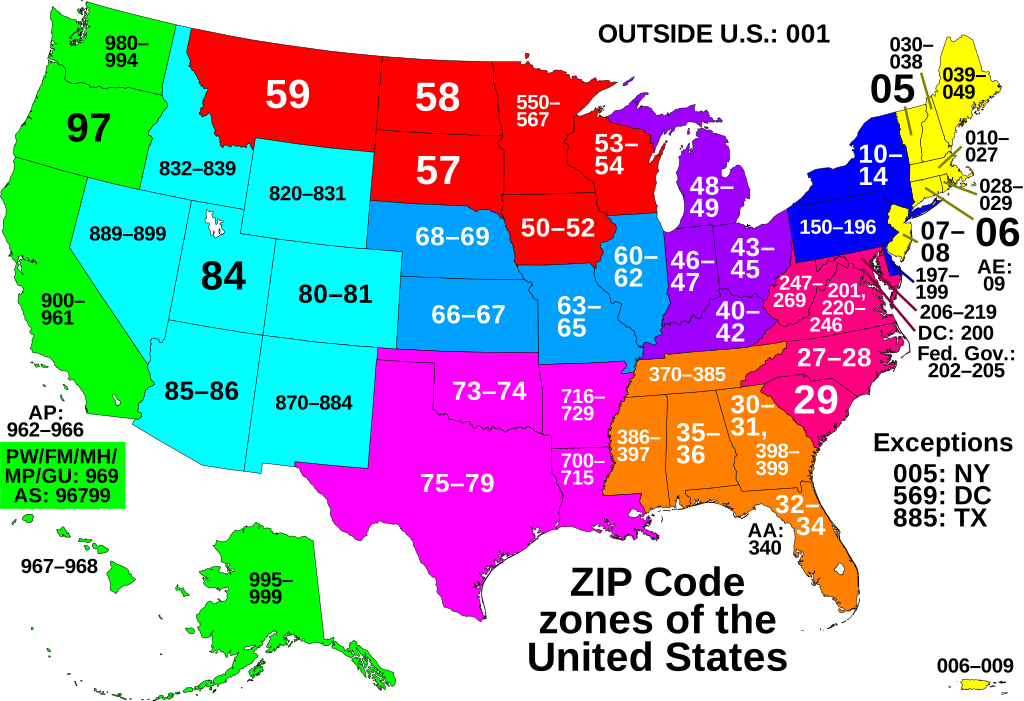
A map that has exceptions baked into the SVG always promises a good story.
A primer on ZIPs↑
Introduced in 1963, ZIP codes are US Postal Service (USPS) routing identifiers used to send and receive mail. If you have an address that receives mail, that address has a ZIP code.
One of the key issues we’ll be discussing in this article is the fundamental problem that ZIP codes describe routes, not areas (or shapes of areas), while GIS-shaped workflows - including SkaldMaps - tend to pretend ZIP codes are areas.
Here’s an example from North Georgia / vaguely Atlanta:
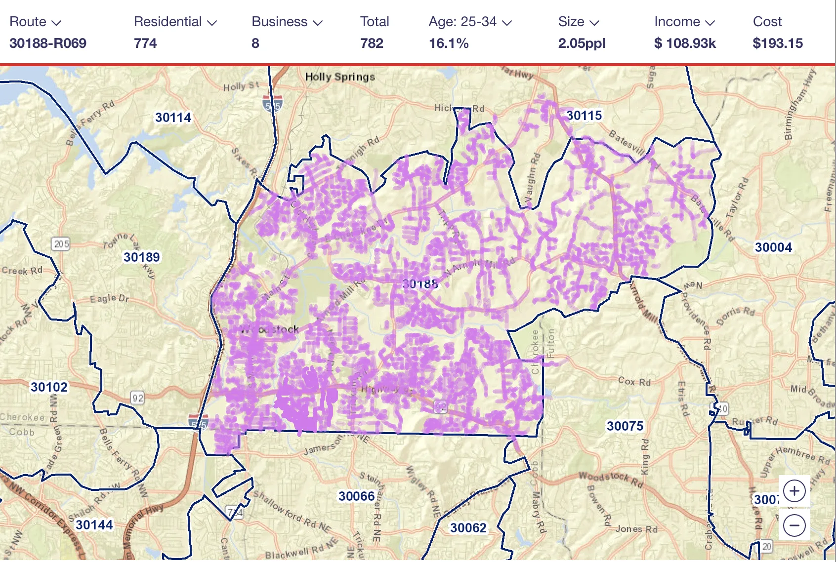
You can see the actual routes on the USPS website.
Any shape of a ZIP (including the one above) we might draw is an approximation - if you’re looking for a house “in” this ZIP code (30188), you’d really be looking for a house with a 30188 address.
Real life, however, doesn’t work like that.
ZIPs have problems↑
But before we jump into the spatial issues, there’s more fun factoids to share that are (if nothing else) interesting to think about:
- ZIP codes are five digits (sometimes with a ZIP+4 extension), but leading zeros matter, so they’re not integers
- ZIP codes can cross city, county, and even state boundaries
- The USPS changes ZIP code definitions over time for operational reasons, so statistical consistency isn’t exactly a given
- Some ZIP codes represent a single building, organization, or PO box facility (or nothing at all)
- Some uninhabited areas don’t have ZIP coverage because there are no mail routes there
- Rural ZIP codes can cover enormous geographic areas, while urban ZIP codes may span only a few blocks
- Perhaps most “fun”: The USPS does not actually maintain an official list of polygons for ZIP codes (for the aforementioned “not a shape” reasons)
A tale of three ZIPs↑
I’m a visual person, so take a look at this (same area as the earlier screenshot):
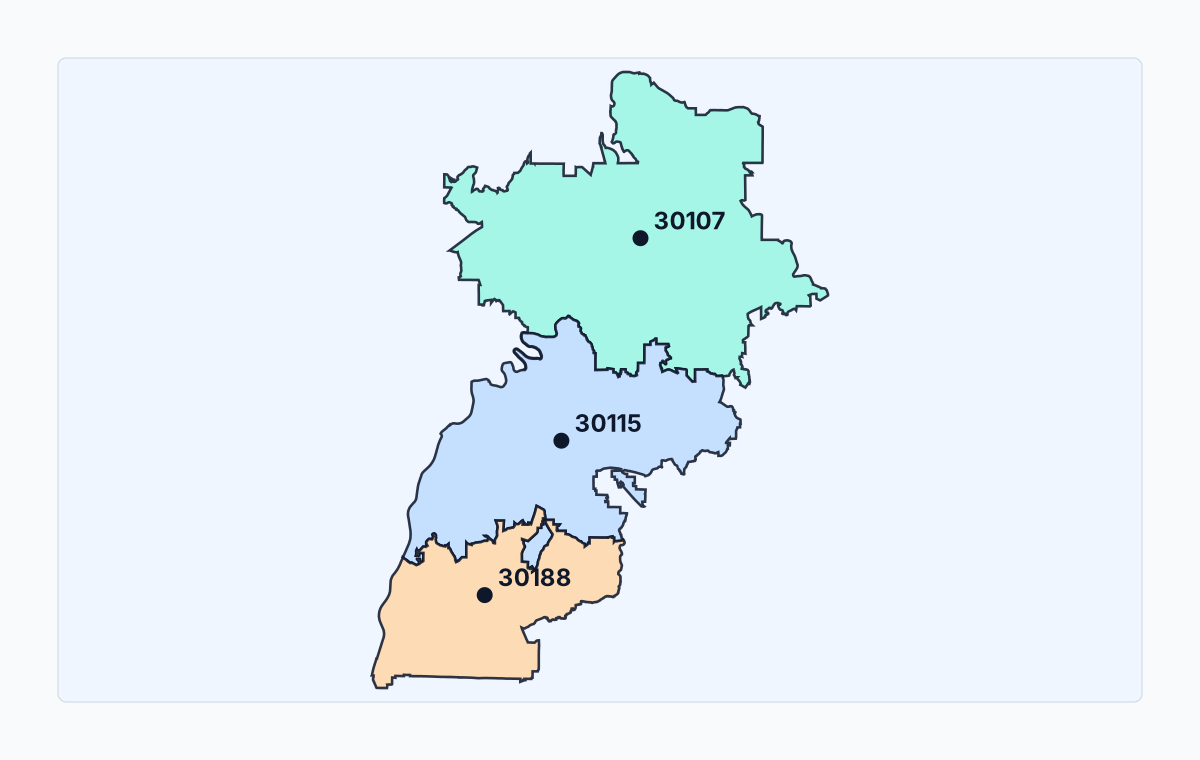
These are three ZIP codes in North GA - they are all somewhat similar by means of proximity, but actually very different between each other, but also within them. These are at the very outer edge of what any reasonable person could consider the “Atlanta metro” (despite the Atlanta–Sandy Springs–Roswell MSA spreading much further, but that’s a rant for another time).
We can see this if we show population density with a bit more detail:
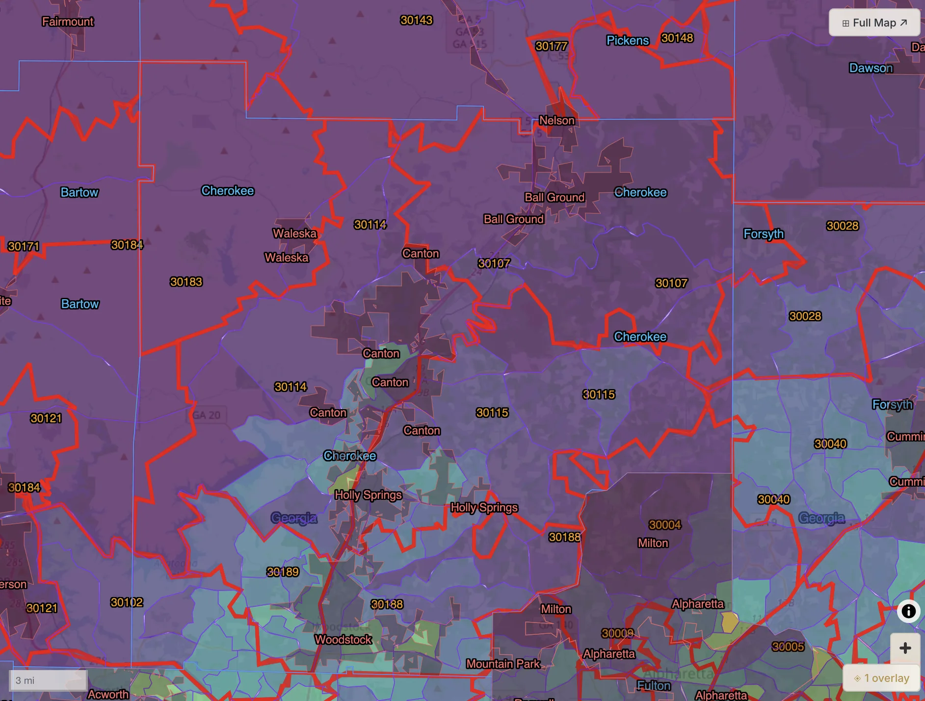
As you can see, the density at the tract level - a separate Census geography, not one level down a ZIP hierarchy - starts to really spike up toward the south (which includes both suburbia as well as “real” cities).
If we zoom into 30188, we can clearly see the city of Woodstock (2020 Census Pop. 35k, but with a dense urban core): A density of up to 3,803 people/sq mi.
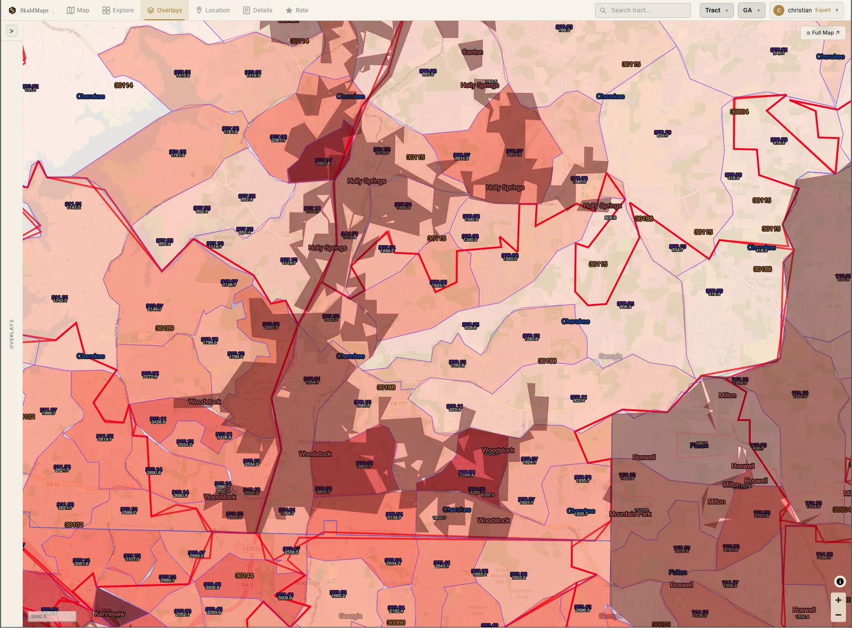
Of course, we can also see the north-eastern parts of this ZIP code going as low as 418 people/sq mi, which works out to over an acre/person (which, for what it’s worth, certainly feels right).
We can visualize this with Google Street View - these two views are part of the same ZIP, less than 15 minutes (or under 7 mi) away from each other.
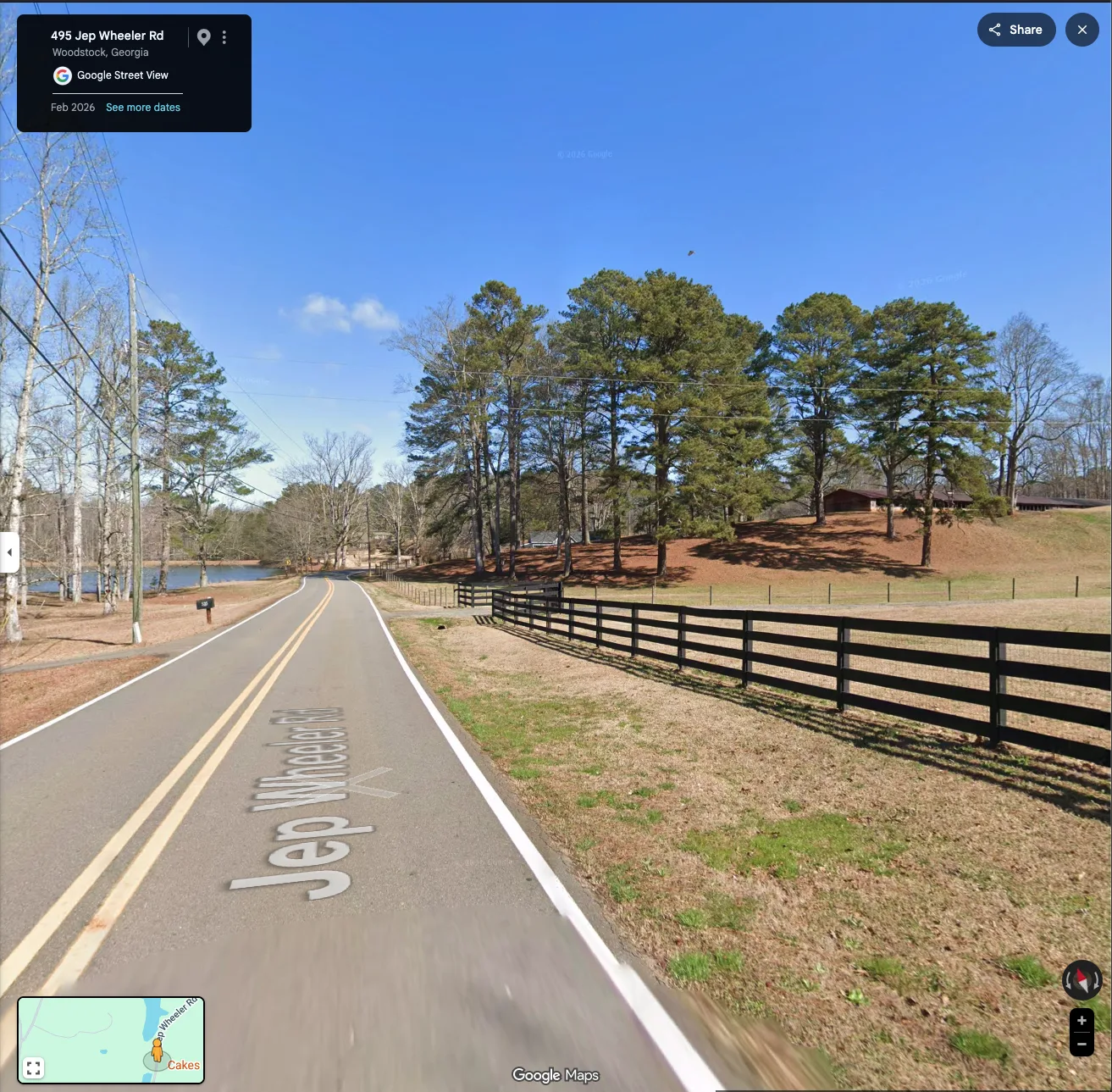
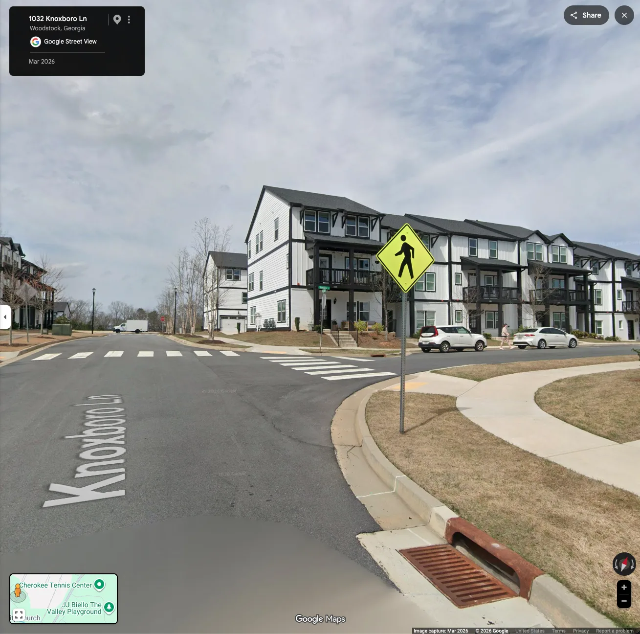
Yet they are both the same ZIP code. And as you can imagine, population density isn’t the only metric that’s different between a small-ish city and an area full of homesteads on acreage.
Usefulness and ubiquity↑
Allow me to slide in a quick SkaldMaps demo to illustrate how we actually use ZIP codes and add context; if you’re not in the mood, skip ahead.
Imagine you’re trying to buy or rent a place.
If we zoom out of our little example and examine the 750+ Georgia ZIP-facing areas in SkaldMaps, we get a much better picture of how much data one must comb through to do just the most basic of pre-filtering to find a place.
If we just pick up the average population density as a metric again and filter for areas > 400 people/sqmi, we can clearly see any (vaguely) urban areas:
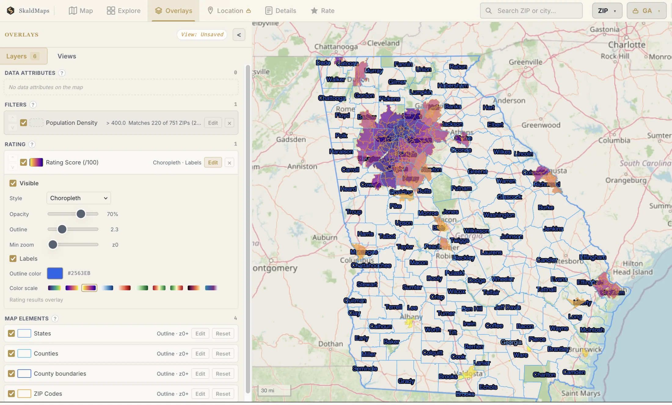
Which, despite not being accurate down to the individual plot, is still a useful view to pre-filter an entire state. Keep in mind that the highlighted area covers millions of people and thousands of square miles. Good luck driving around all that looking for realtor signs! (Yes, this is a “traffic in Atlanta is a nightmare” reference.)
While filtering (or rating on) density is a relatively trivial task, we can add more layers to this.
Say, for instance, I’m looking for a place within 25 mi of Woodstock, GA (moving for work, for instance) but I desperately need premium retail shopping in my life and want a high share of 4+ bedroom houses to house a large family, we can visualize that:
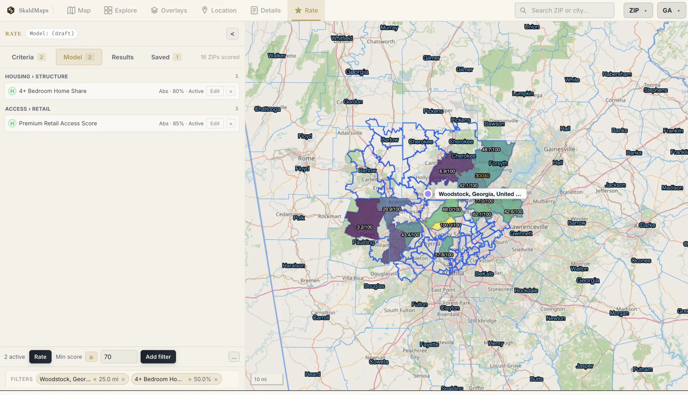
The resulting 16 ZIPs that survive the 25 mile location filter are all still vastly different; we can now iterate on this model (and filters) to really shortlist areas to search in. We also offer helpful details, statistics, and distributions per ZIP to help make sense of any ZIP.
In this example, 30068 in Cobb County has scored the best, so we could use that to search for a place to buy and look into the details there:
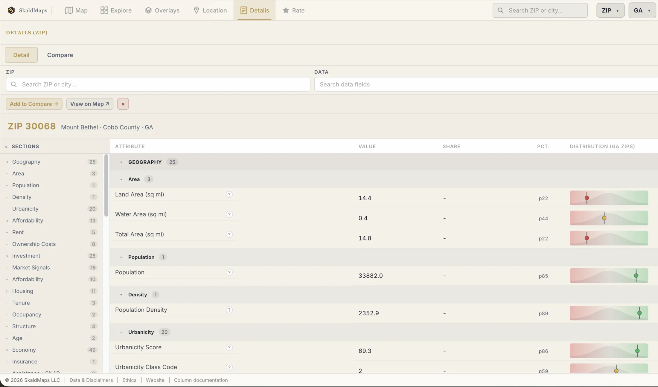
This detailled view shows us statistics - such as distribution compared to the rest of the state - which adds much needed context to the “raw” data we have on a given ZIP code.
For completeness’ sake, 30068 is reasonably consistent (unlike the example from earlier), which we can see on the tract level:
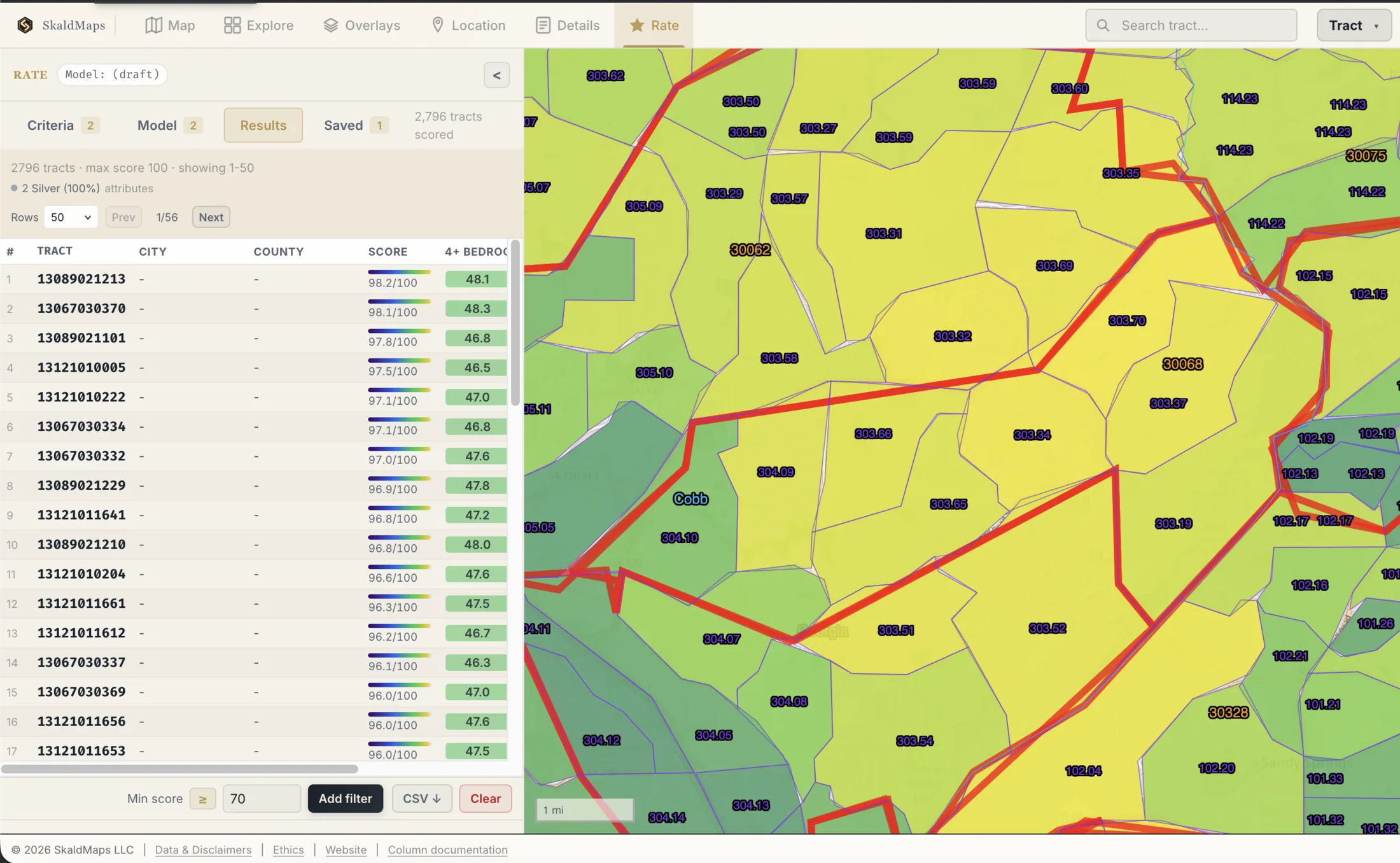
Which is also why the ZIP codes around 30068 largely scored well.
We can now take this ZIP and actually look for places on an MLS marketplace of our choosing; in July 2026, there were 144 houses for sale on Zillow in that area, which is a much more manageable scope to actually shop for than trying to tackle the entire metro Atlanta real estate market at once.
ZIP codes are everywhere↑
The previous link to Zillow illustrates this well: ZIP codes are everywhere: Major RE portals (including MLS systems directly) support them as a first-class citizen because, by and large, they are good enough.
They are also standardized (which isn’t the same as “consistent”), whereas things like “neighborhoods” are very much subjective.
This is easy in some places: NYC, for instance, has arguably very well-defined neighborhoods and most people will agree where “Hell’s Kitchen” is located (which is defined by street names, but Wikipedia also lists three ZIP codes: 10018, 10019, and 10036). NYC is also very densely populated, so the ZIP codes there are tiny.
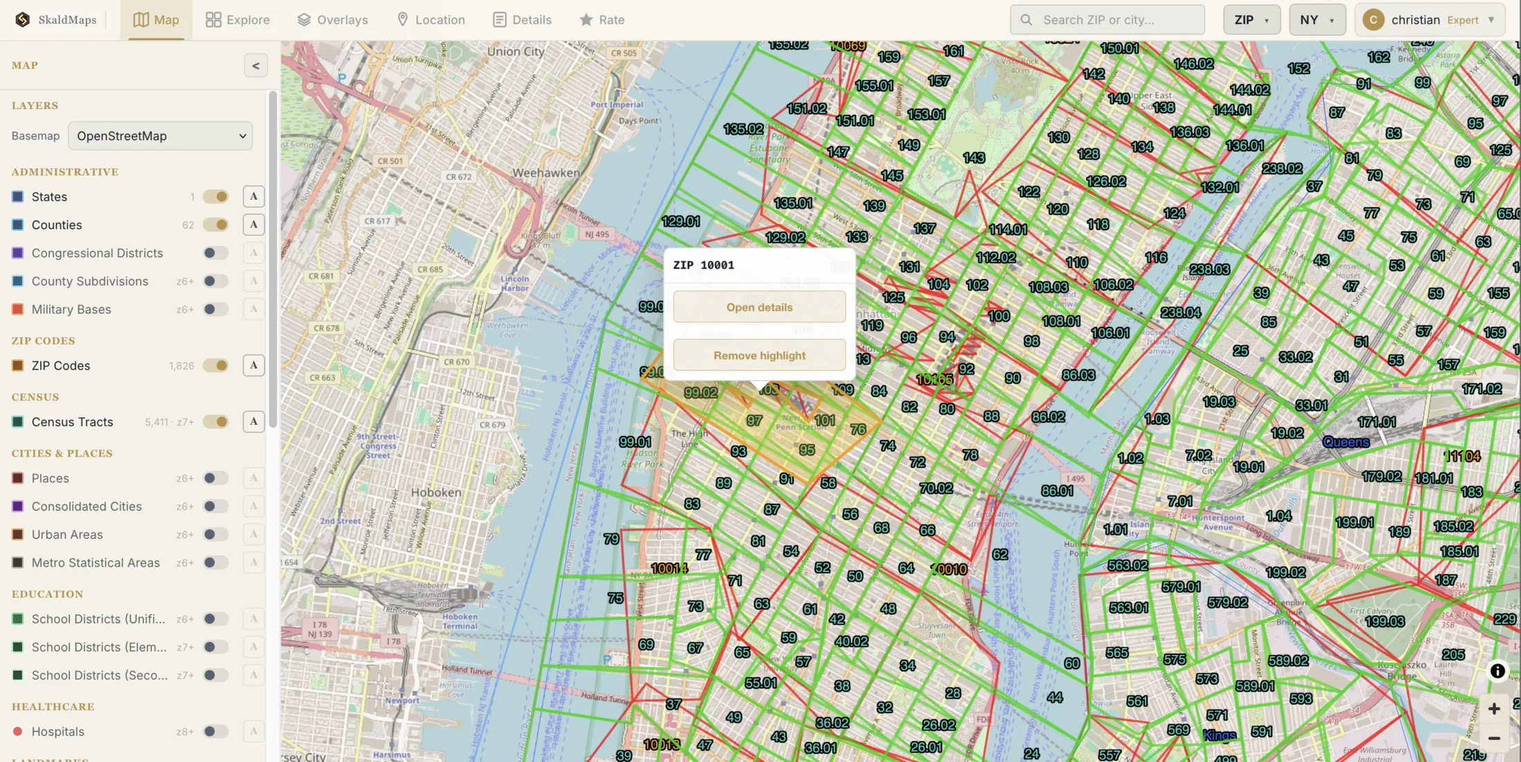
I can’t say the same thing about Atlanta - you’d be hard pressed to find two people that agree on where “metro” Atlanta starts and ends (which culturally isn’t the same as just looking at the MSA overlay), not to mention neighborhoods.
We can, however, largely agree where 30188 is on the map and find houses there, if we so desire. We can also reasonably declare that 30188 is very different to 31011 (primarily in Dodge County, GA, with a 2024 ACS 5-year estimated population of roughly 500).
So is using ZIPs for things they weren’t designed for a good thing? Well, no. Is it a realistic thing - as in, does the real world work like that? Well, yes.
…which is why we use them on SkaldMaps. But how do we make ZIPs work if they’re so horrible?
ZCTAs, Tracts, and Crosswalks↑
A side note: DuckDB 🦆↑
SkaldMaps uses
DuckDB with the SPATIAL extension behind the scenes.
Any SQL below is DuckDB’s SQL dialect, which is similar to PostgreSQL. And I’ll let you in on another engineering secret: We also use Postgres.
If you’re familiar with both data engineering (or data science) and geospatial work, you’ll know how fantastic DuckDB is. If not, we’ll run an article on how we use DuckDB shortly! We won’t do any SQL deep dives here, but it’s useful context to understand how we make it work.
And as a final note, the non-SkaldMaps screenshots and graphs here were done with the wonderful marimo.
ZIP and tract native data↑
ZIPs aren’t great, so before we show you ZIP-level data, we work with the most useful native geography a source gives us; for ACS, our fine-grained layer is Census tracts.
A very popular (and very large) dataset comes from the ACS, the American Community Survey, run by the US Census Bureau. They have a lot of data.
The Census - being all about statistics - publishes data at a lot of levels. For ACS 5-year estimates, block groups are smaller than tracts; SkaldMaps uses tracts as its fine-grained layer because they offer a useful balance of detail, nationwide coverage, and stability.
SkaldMaps uses, among other datasets, the ACS; in fact, most RE software / geospatial tools do.
ACS 5-year data is relatively simple, since it’s published on both a tract and ZCTA (“ZIP”) level. I’m not saying we don’t have to do anything with the raw data (we do - I should know, since I did it!), but it’s very pleasant.
For instance, this is what one of the raw ACS 5-year files looks like:
| GEO_ID | NAME | S1701_C02_001E | S1701_C03_001E |
|---|---|---|---|
| Geography | Geographic Area Name | Estimate!!Below poverty level!!Population for whom poverty status is determined | Estimate!!Percent below poverty level!!Population for whom poverty status is determined |
| 1400000US13057090809 | Census Tract 908.09, Cherokee County, Georgia | 214 | 5.8 |
And on a ZCTA level:
| GEO_ID | NAME | S1701_C02_001E | S1701_C03_001E |
|---|---|---|---|
| Geography | Geographic Area Name | Estimate!!Below poverty level!!Population for whom poverty status is determined | Estimate!!Percent below poverty level!!Population for whom poverty status is determined |
| 8600000US30188 | ZCTA5 30188 | 3900 | 6.1 |
The ZCTA covers 47.4% of the area of Census Tract 908.09. That does not mean that 47.4% of the tract’s 214 people below the poverty level live in 30188: People aren’t spread evenly for our convenience, and the ZCTA also overlaps many other tracts.
Fortunately, this is ACS data, so the Census already gives us the ZCTA estimate directly: 3,900 people, or 6.1%. We don’t need to invent it from the overlap.
Once you visualize the actual areas, you can maybe make a little more sense of it:
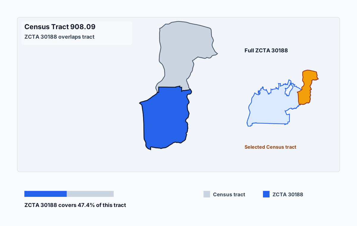
So we can natively display both, as the work is done for us by the Census Bureau. For ZIP metrics, we use the ZCTA row directly rather than calculating it from tract rows. We also get data points like margin of error, but don’t yet surface them in the application.
Crosswalks↑
But ACS data is easy, since we get it more or less directly from the source and show ZIP-shaped data. What happens if useful data is published only for tracts or counties, but we want a ZIP view?
HUD publishes the HUD-USPS ZIP Code Crosswalk Files for exactly this problem. They are derived from quarterly USPS address data: For every ZIP/Census-geography pair, they count residential, business, other, and total addresses, then publish each count as a ratio.
That is useful because it follows where people and businesses actually receive mail, since a dense subdivision and large (but empty) timber tracts are very different places (usually more deer on the latter).
They come in two flavors: Tract-to-ZIP and ZIP-to-tract. The first answers “What share of this tract’s addresses belongs to this ZIP?”; the second answers “Where do this ZIP’s addresses fall?”.
We keep both directions and, for housing and resident-facing measures, largely use the residential address ratio.
This is how we turn a tract-level count into a ZIP-facing estimate: If tract A has 1,000 occupied homes and the tract-to-ZIP crosswalk says 25% of its residential addresses belong to ZIP 30115, we allocate 250 homes to 30115. We repeat that for every overlapping tract, then add the allocated counts together.
That does not make tracts and ZIPs interchangeable, but it is useful for additive facts such as people, homes, or votes (although voting data is a whole new rabbit hole unrelated to the ACS).
For rates we can rebuild from their allocated numerator and denominator; however, it does not make a tract-level median home value or percentile magically reversible.
Once again, we’ll go back to our ZIP codes from earlier, since this is easiest visualized by picking an example: Tracts overlap with ZIP codes. They aren’t related, but we can measure a relationship.
Here’s an example (fun fact, the darkest tract here is a giant subdivison, but also happens to include places on acreage, since tracts aren’t neighborhoods - see above):
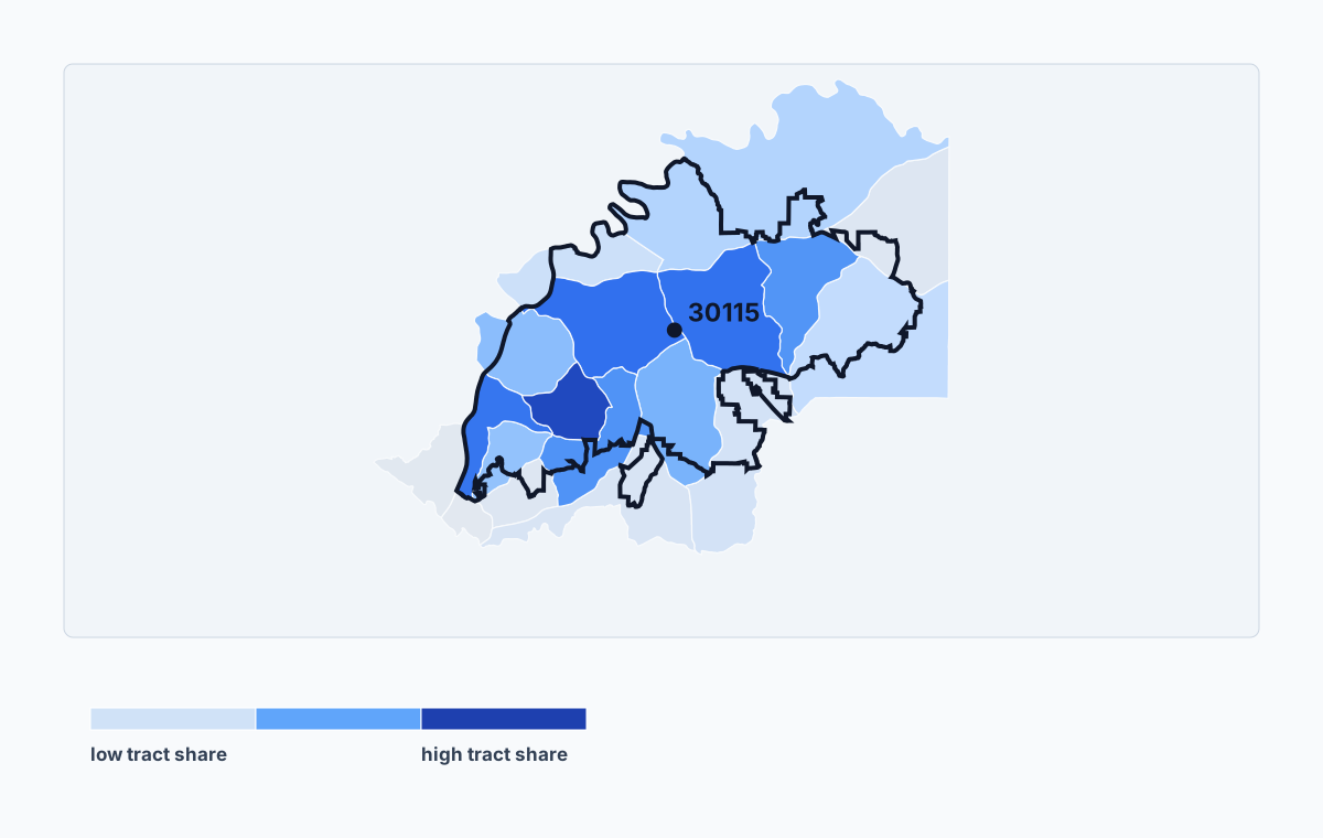
Using the tract-to-ZIP file, the relevant residential address weight is just a bit of SQL to illustrate:
SELECT tract_fips, res_ratio AS tract_to_zip_residential_weightFROM read_csv_auto('usps_tract_zip_crosswalk.csv')WHERE zip = '30115'ORDER BY tract_to_zip_residential_weight DESC;┌─────────────┬─────────────────────────────────┐│ tract_fips │ tract_to_zip_residential_weight ││ varchar │ double │├─────────────┼─────────────────────────────────┤│ 13057090807 │ 1.0 ││ 13057090603 │ 1.0 ││ 13057090504 │ 1.0 ││ 13057090703 │ 0.9987466053349001 ││ 13057090505 │ 0.9983388744417365 ││ 13057090810 │ 0.7786298568507157 │Each row says what share of that tract’s residential addresses belongs to 30115. For the reverse question, we can use the ZIP-to-tract version instead.
This is why crosswalks are useful for us: They let an address-based ZIP act as a reasonable presentation layer for data collected on a different Census geography.
Manually approximating geometries↑
But what if that isn’t an option and we just have geometries?
The missing piece here is Census TIGER/Line shapefiles (“Topologically Integrated Geographic Encoding and Referencing”) that give us published boundary geometries.
So with those, fear not, we can do something similar, albeit with a different methodology. While crosswalk files estimate relationships from address counts, geometries let us estimate relationships from physical overlap. We use this for polygon sources and as a flagged fallback when a crosswalk is unavailable; where a population estimate is appropriate and available, we use that, too.
This is a form of areal interpolation. One caveat in our current fallback is that TIGER’s longitude/latitude coordinates are not an equal-area projection. Ratios between nearby pieces are often useful, but they are not true equal-area measurements, so we treat them as approximations; a more rigorous calculation projects both layers to the same suitable equal-area CRS first.
Spatial overlap can be a good strategy, too. Here’s another example of a specific type of overlap (in this case, urban area tracts):
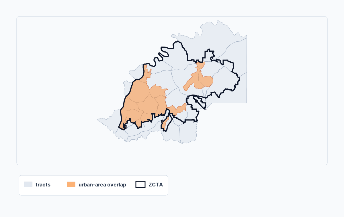
Remember, tracts and ZIPs aren’t related and overlap wildly.
We can, however, intersect shapes and see what overlaps (and by how much and how it does so). This conceptually works for any shape, not just tract/census data.
Behold, more SQL - this time showing the more rigorous equal-area version:
WITH overlaps AS (    SELECT        z.zip,        t.tract_fips,        -- SPATIAL magic! These fields were projected to the same        -- equal-area CRS before this query.        ST_Area(ST_Intersection(z.equal_area_geom, t.equal_area_geom)) AS overlap_area    FROM zip AS z    JOIN tract AS t        ON z.statefp = t.statefp        AND ST_Intersects(z.equal_area_geom, t.equal_area_geom)    WHERE z.zip = '30115')
SELECT    zip,    tract_fips,    overlap_area        / SUM(overlap_area) OVER (PARTITION BY zip) AS tract_share_of_zipFROM overlapsORDER BY tract_share_of_zip DESC;
If a metric is additive - e.g., people, households, votes, enrolled students, and so on - we can allocate the relevant pieces and then rebuild the ZIP-facing number.
We generally don’t want to average percentages directly. If one tract has 100 people and another has 10,000 people, those two percentages should not count the same. Instead, we allocate the numerator and denominator, then recompute the percentage at the ZIP level.
That isn’t the same as what the crosswalk files do, but it’s a decent approximation.
It also comes with the usual GIS caveats: changing the boundaries can change the answer (the modifiable areal unit problem), and an area-wide estimate says nothing certain about any individual inside it (the ecological fallacy).
Since this is a bit abstract, here’s an actual example. Our Census Urban Area Coverage metric first measures what share of each tract is covered by Census urban-area polygons (which is part of the “Urbanicity” attribute, which is one of our custom attributes), then rolls those tract shares up to a ZIP:
Tract Urban Area Coverage =  area(tract ∩ Census urban areas) / area(tract)
ZIP Census Urban Area Coverage =  sum(tract urban-area coverage * ZIP-to-tract weight)  / sum(ZIP-to-tract weight)
ZIP 30115 = 62.8%
The geometric overlap gives us the tract-level fact; the ZIP-to-tract weights keep the ZIP rollup from treating every tract as equally important.
This isn’t exact, but it’s pretty good for many attributes.
Points aren’t great, either↑
So we’ve established that ACS native data is easy to deal with, we can use crosswalk data to translate Census related data, and we can use shapes to approximate spatial attributes that are unrelated to the Census. Non-ACS data isn’t an edge case for us: 134 of our current 301 app-visible attributes are not plain ACS rows. But those sources aren’t always polygons. What about points?
Amenities and points of interest have a different problem. A hospital, park, airport, grocery store (or any business location) is a point - as in, it’s quite literally a tuple of coordinates whose meaning depends on its coordinate system. GeoJSON makes that explicit: it uses WGS 84. No, I don’t love that, but it is what it is.
Expressed in GeoJSON:
{ "type": "Point", "coordinates": [30.0, 10.0]}And, as we’ve established, tracts/ZIPs… are, sort of, geometries (polygons).
An example: Hospitals in Michigan↑
For SkaldMaps, we have 2 main use cases that deal with points and ZIPs:
- Count points that fall inside the ZCTA boundary (“How many hospitals are in this ZIP/County?”)
- Measure distance from the ZCTA’s Census internal point to nearby points (“How many amenities are nearby/within 15, 25, or 50 miles?”).
Both are useful, both aren’t something a lot of tools do, but both are… challenging. Largely because the real world is challenging.
If you ask any “Where is point X in relation to this ZIP?” (or county or tract level, for that matter - in other words, for any polygon) question, a common way of answering that is by using the centroid of the polygon, i.e. the mathematical center. SkaldMaps instead uses Census-published internal points where available (this doesn’t help if we have polygons that aren’t related to the Census). That avoids some weird polygon-center failures, but it is still only one point standing in for an entire area.
If you don’t think that’s misleading, remember for a second that Alaska and Hawaii exist and ask where the geographic center of the entire country is. Spoiler, it’s not Kansas:
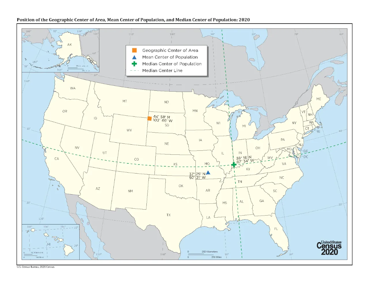
Which is correct, but largely useless for everyday use (a conventional geographic center of the lower 48 is near Lebanon, Kansas, though).
Here’s a more local example, this time from Michigan; even with an internal point, the same one-point problem persists - it isn’t necessarily intuitive and might be far away from where you actually are.
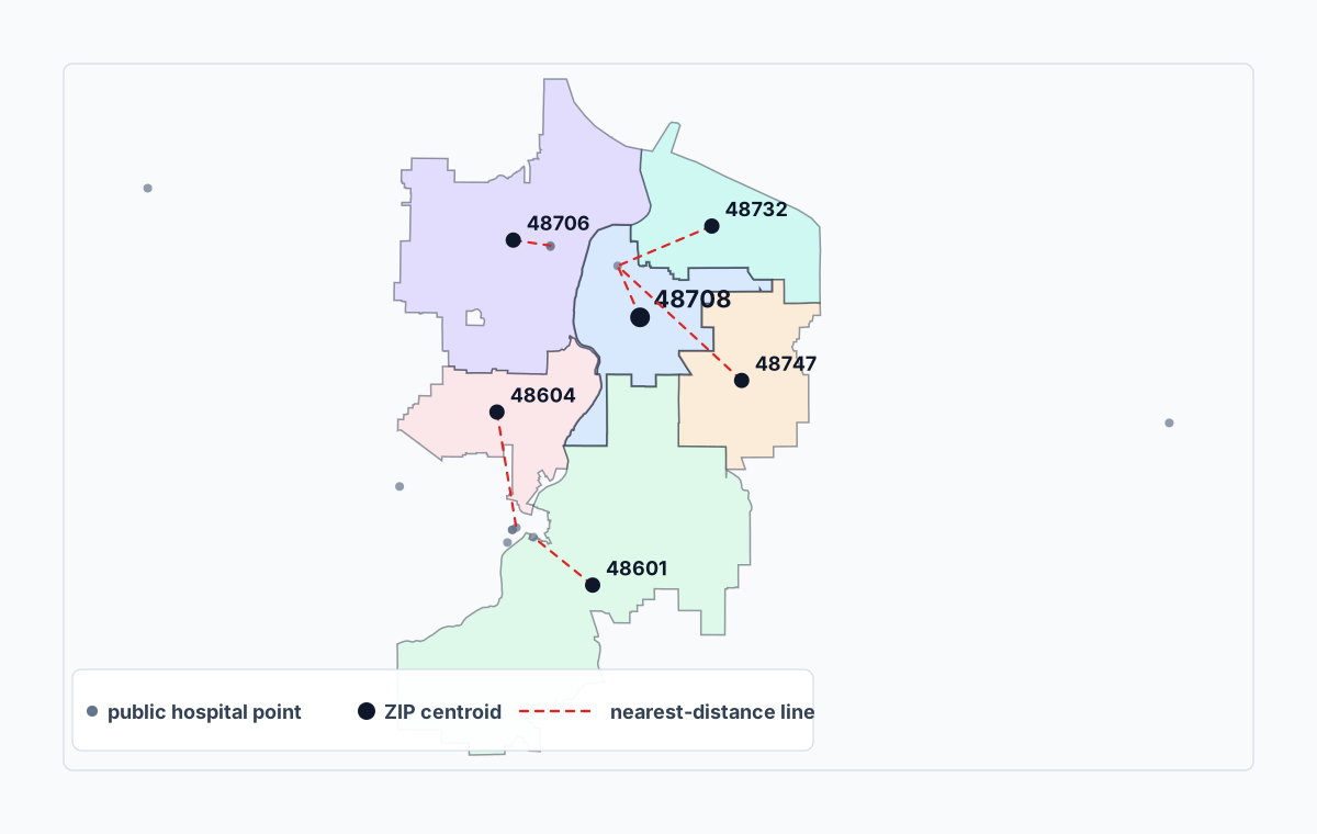
In this example, the 5 top ZIP codes are Bay City, MI, mapped to healthcare amenities. Four of them point to the McLaren Bay Region Hospital in Bay City, which makes a lot of sense.
However, the internal point for ZIP code 48601 - a 104-square-mile area - is really closer to Saginaw, the city to the south. Take a look at this screenshot from SkaldMaps:
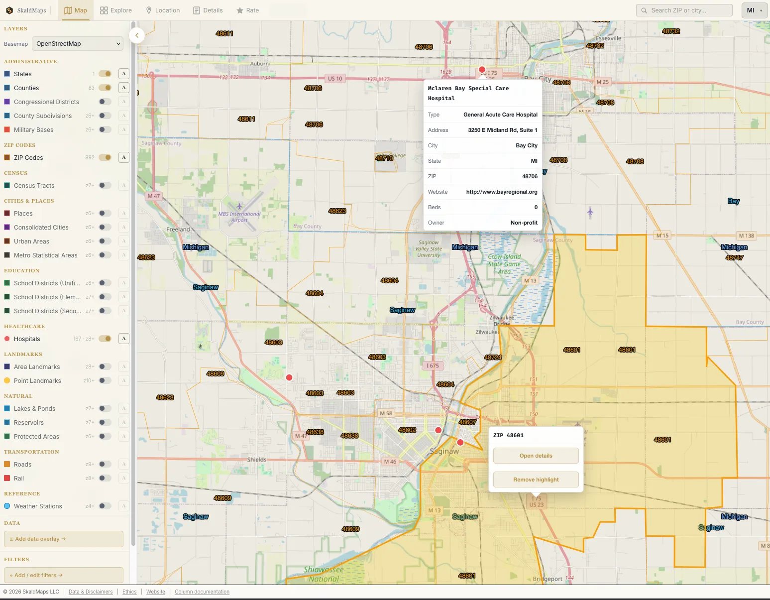
You can clearly see the cluster of healthcare amenities in Saginaw. But if you live in the northern part of 48601, that information isn’t really that accurate for you.
What are we doing about it?↑
My hot take is: The question of “what’s the nearest hospital to 48601” is just a bad question in isolation. It can be a great part of a rating model or any general purpose analysis, however, especially combined with other variables.
So, SkaldMaps lets you do a few things with points. To re-use the hospital idea:
- “How far is the nearest hospital?” answers this on an internal-point basis, which is imperfect, but at least gives you an idea (that’s what we did earlier)
- “What is the nearest hospital?” adds context as non-numeric metadata to the result; even if using internal-point distance is slightly misleading, we can show you the details of the hospital
- “How many hospitals are within 15/25/50 miles?” gives you more useful context than a single facility, although it still shares the one-point limitation
And, naturally, you can combine this with things like population density, location context, etc.
For instance, plotting “Nearest Hospital” across the lower part of the state, we are met with a reasonably useful choropleth:
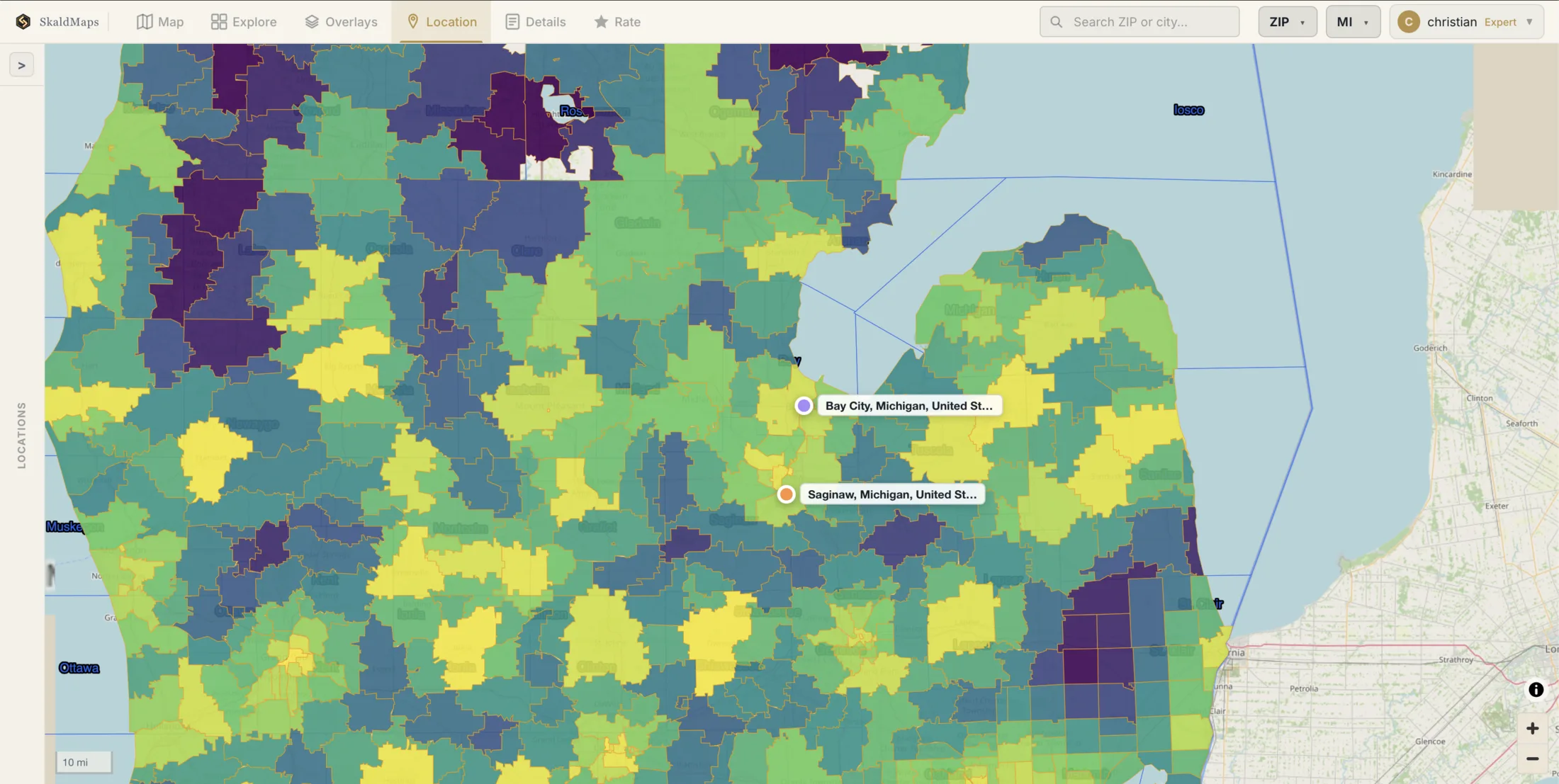
And once we find a ZIP that’s interesting (such as 48601 from before), we can use the details view to answer question #2, telling us details about the actual hospital in question, as well as question #3 (how many hospitals are around the ZIP’s internal point)?
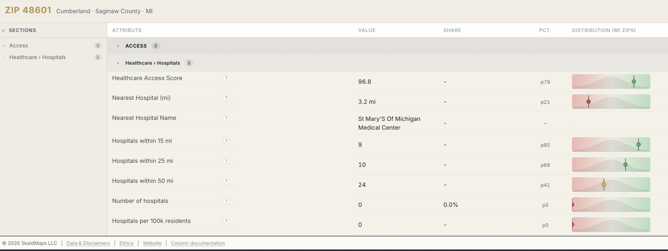
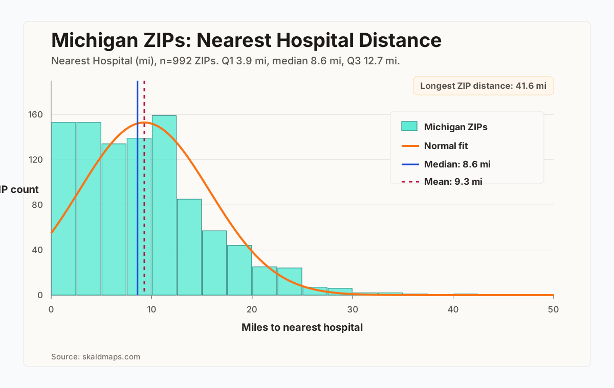
This view also provides additional context: That ZIP’s (again, flawed) nearest-hospital distance (3.2 mi) puts it at p21 across the entire state, which is great.
The p95 distance, including Michigan’s largely rural Upper Peninsula, is 21.5 mi.
In fact, here’s a distribution graph:
Functionally, this sort of works like this:
SET geometry_always_xy = false;
WITH distances AS (    SELECT        z.zip,        h.name AS hospital_name,        ST_Distance_Sphere(            ST_Point(z.lat, z.lon),            ST_Point(h.lat, h.lon)        ) / 1609.344 AS distance_miles -- simplified to horrify metric enjoyers    FROM zips AS z    CROSS JOIN hospitals AS h    WHERE z.zip = '48601')
SELECT zip, arg_min(hospital_name, distance_miles) AS nearest_hospital, min(distance_miles) AS nearest_hospital_miles, count_if(distance_miles <= 15) AS hospitals_within_15mi, count_if(distance_miles <= 25) AS hospitals_within_25mi, count_if(distance_miles <= 50) AS hospitals_within_50miFROM distancesGROUP BY zip;Conclusion↑
ZIP codes are bad default units for spatial statistics (and if you talk to a mathematician, all statistics are bad math, and then it’s turtles all the way down and we should all forage for mushrooms, but I digress). They are also, annoyingly, the geography normal people actually use.
We hedge against all the issues ZIP codes have with a few strategies:
- We start at each source’s native grain - ACS, weather, healthcare, education, housing, voting, and more - rather than treating every input as a ZIP table
- When mapping data to a target geography, we try to use crosswalk files; if we can’t, we use the appropriate documented spatial or point-based approximation
- We are reasonably transparent about how we derive a metric and give you a confidence indicator (and blog about it), so you can judge for yourself how much you want to trust a metric
- We offer you the ability to combine many metrics and attributes in our rating engine, without pretending that an aggregate score removes uncertainty in its inputs
- We provide a detailed view, including distributions and non-numeric metadata that add context
- You can always ask if something is unclear ❤️
So, yes, we are aware: ZIP codes suck. But I also hope this article clarified that we are, in fact, aware of this and, more importantly, how we work around it.